Simpson's paradox
In probability and statistics, Simpson's paradox (or the Yule–Simpson effect) is a paradox in which a correlation present in different groups is reversed when the groups are combined. This result is often encountered in social-science and medical-science statistics,[1] and it occurs when frequency data are hastily given causal interpretations.[2] Simpson's Paradox disappears when causal relations are brought into consideration (see Implications to decision making).
Though it is mostly unknown to laymen, Simpson's Paradox is well known to statisticians, and it is described in a few introductory statistics books.[3][4] Many statisticians believe that the mainstream public should be informed of the counter-intuitive results in statistics such as Simpson's paradox.[5][6]
Edward H. Simpson first described this phenomenon in a technical paper in 1951,[7] but the statisticians Karl Pearson, et al., in 1899,[8] and Udny Yule, in 1903, had mentioned similar effects earlier.[9] The name Simpson's paradox was introduced by Colin R. Blyth in 1972.[10] Since Edward Simpson did not actually discover this statistical paradox,[note 1] some writers, instead, have used the impersonal names reversal paradox and amalgamation paradox in referring to what is now called Simpson's Paradox and the Yule-Simpson effect.[11]
Contents |
Examples
Civil Rights Act of 1964
A real-life example is the passage of the Civil Rights Act of 1964 in the United States. Overall, a larger fraction of Republican legislators voted in favor of the Act than Democrats. However, when the congressional delegations from the northern and southern States are considered separately, a larger fraction of Democrats voted in favor of the act in both regions. This arose because regional affiliation is a very strong indicator of how a congressman or senator voted, but party affiliation is a weak indicator.
| House | Democrat | Republican |
|---|---|---|
| Northern | 94% (145/154) | 85% (138/162) |
| Southern | 7% (7/94) | 0% (0/10) |
| Both | 61% (152/248) | 80% (138/172) |
| Senate | Democrat | Republican |
|---|---|---|
| Northern | 98% (45/46) | 84% (27/32) |
| Southern | 5% (1/21) | 0% (0/1) |
| Both | 69% (46/67) | 82% (27/33) |
Kidney stone treatment
This is another real-life example from a medical study[12] comparing the success rates of two treatments for kidney stones.[13]
The table shows the success rates and numbers of treatments for treatments involving both small and large kidney stones, where Treatment A includes all open procedures and Treatment B is percutaneous nephrolithotomy:
| Treatment A | Treatment B | |
|---|---|---|
| Small Stones | Group 1 93% (81/87) |
Group 2 87% (234/270) |
| Large Stones | Group 3 73% (192/263) |
Group 4 69% (55/80) |
| Both | 78% (273/350) | 83% (289/350) |
The paradoxical conclusion is that treatment A is more effective when used on small stones, and also when used on large stones, yet treatment B is more effective when considering both sizes at the same time. In this example the "lurking" variable (or confounding variable) of the stone size was not previously known to be important until its effects were included.
Which treatment is considered better is determined by an inequality between two ratios (successes/total). The reversal of the inequality between the ratios, which creates Simpson's paradox, happens because two effects occur together:
- The sizes of the groups, which are combined when the lurking variable is ignored, are very different. Doctors tend to give the severe cases (large stones) the better treatment (A), and the milder cases (small stones) the inferior treatment (B). Therefore, the totals are dominated by groups three and two, and not by the two much smaller groups one and four.
- The lurking variable has a large effect on the ratios, i.e. the success rate is more strongly influenced by the severity of the case than by the choice of treatment. Therefore, the group of patients with large stones using treatment A (group three) does worse than the group with small stones, even if the latter used the inferior treatment B (group two).
Berkeley gender bias case
One of the best known real life examples of Simpson's paradox occurred when the University of California, Berkeley was sued for bias against women who had applied for admission to graduate schools there. The admission figures for the fall of 1973 showed that men applying were more likely than women to be admitted, and the difference was so large that it was unlikely to be due to chance.[3][14]
| Applicants | Admitted | |
|---|---|---|
| Men | 8442 | 44% |
| Women | 4321 | 35% |
But when examining the individual departments, it appeared that no department was significantly biased against women. In fact, most departments had a "small but statistically significant bias in favor of women."[14] The data from the six largest departments are listed below.
| Department | Men | Women | ||
|---|---|---|---|---|
| Applicants | Admitted | Applicants | Admitted | |
| A | 825 | 62% | 108 | 82% |
| B | 560 | 63% | 25 | 68% |
| C | 325 | 37% | 593 | 34% |
| D | 417 | 33% | 375 | 35% |
| E | 191 | 28% | 393 | 24% |
| F | 272 | 6% | 341 | 7% |
The research paper by Bickel, et al.[14] concluded that women tended to apply to competitive departments with low rates of admission even among qualified applicants (such as in the English Department), whereas men tended to apply to less-competitive departments with high rates of admission among the qualified applicants (such as in engineering and chemistry). The conditions under which the admissions' frequency data from specific departments constitute a proper defense against charges of discrimination are formulated in the book Causality by Pearl.[2]
Low birth weight paradox
The low birth weight paradox is an apparently paradoxical observation relating to the birth weights and mortality of children born to tobacco smoking mothers. As a usual practice, babies weighing less than a certain amount (which varies between different countries) have been classified as having low birth weight. In a given population, babies with low birth weights have had a significantly higher infant mortality rate than others. However, it has been observed that babies of low birth weights born to smoking mothers have a lower mortality rate than the babies of low birth weights of non-smokers.[15]
Batting averages
A common example of Simpson's Paradox involves the batting averages of players in professional baseball. It is possible for one player to hit for a higher batting average than another player during a given year, and to do so again during the next year, but to have a lower batting average when the two years are combined. This phenomenon can occur when there are large differences in the number of at-bats between the years. (The same situation applies to calculating batting averages for the first half of the baseball season, and during the second half, and then combining all of the data for the season's batting average.)
A real-life example is provided by Ken Ross[16] and involves the batting average of two baseball players, Derek Jeter and David Justice, during the baseball years 1995 and 1996:[17]
| 1995 | 1996 | Combined | ||||
|---|---|---|---|---|---|---|
| Derek Jeter | 12/48 | .250 | 183/582 | .314 | 195/630 | .310 |
| David Justice | 104/411 | .253 | 45/140 | .321 | 149/551 | .270 |
In both 1995 and 1996, Justice had a higher batting average (in bold type) than Jeter did. However, when the two baseball seasons are combined, Jeter shows a higher batting average than Justice. According to Ross, this phenomenon would be observed about once per year among the possible pairs of interesting baseball players. In this particular case, the Simpson's Paradox can still be observed if the year 1997 is also taken into account:
| 1995 | 1996 | 1997 | Combined | |||||
|---|---|---|---|---|---|---|---|---|
| Derek Jeter | 12/48 | .250 | 183/582 | .314 | 190/654 | .291 | 385/1284 | .300 |
| David Justice | 104/411 | .253 | 45/140 | .321 | 163/495 | .329 | 312/1046 | .298 |
The Jeter and Justice example of Simpson's paradox was referred to in the "Conspiracy Theory" episode of the television series Numb3rs, though a chart shown omitted some of the data, and listed the 1996 averages as 1995.
Description
Suppose two people, Lisa and Bart, each edit document articles for two weeks. In the first week, Lisa improves 60% of the 100 articles she edited, and Bart improves 90% of 10 articles he edited. In the second week, Lisa improves just 10% of 10 articles she edited, while Bart improves 30% of 100 articles he edited.
| Week 1 | Week 2 | Total | |
|---|---|---|---|
| Lisa | 60/100 | 1/10 | 61/110 |
| Bart | 9/10 | 30/100 | 39/110 |
Both times Bart improved a higher percentage of articles than Lisa, but the actual number of articles each edited (the bottom number of their ratios also known as the sample size) were not the same for both of them either week. When the totals for the two weeks are added together, Bart and Lisa's work can be judged from an equal sample size, i.e. the same number of articles edited by each. Looked at in this more accurate manner, Lisa's ratio is higher and, therefore, so is her percentage. Also when the two tests are combined using a weighted average, overall, Lisa has improved a much higher percentage than Bart because the quality modifier had a significantly higher percentage. Therefore, like other paradoxes, it only appears to be a paradox because of incorrect assumptions, incomplete or misguided information, or a lack of understanding a particular concept.
| Week 1 quantity | Week 2 quantity | Total quantity and weighted quality | |
|---|---|---|---|
| Lisa | 60% | 10% | 55.5% |
| Bart | 90% | 30% | 35.5% |
This imagined paradox is caused when the percentage is provided but not the ratio. In this example, if only the 90% in the first week for Bart was provided but not the ratio (9:10), it would distort the information causing the imagined paradox. Even though Bart's percentage is higher for the first and second week, when two weeks of articles is combined, overall Lisa had improved a greater proportion, 55% of the 110 total articles. Lisa's proportional total of articles improved exceeds Bart's total.
Here are some notations:
- In the first week
-
 — Lisa improved 60% of the many articles she edited.
 — Bart had a 90% success rate during that time.
- Success is associated with Bart.
- In the second week
-
 — Lisa managed 10% in her busy life.
 — Bart achieved a 30% success rate.
- Success is associated with Bart.
On both occasions Bart's edits were more successful than Lisa's. But if we combine the two sets, we see that Lisa and Bart both edited 110 articles, and:
 — Lisa improved 61 articles.
 — Bart improved only 39.
 — Success is now associated with Lisa.
Bart is better for each set but worse overall.
The paradox stems from the intuition that Bart could not possibly be a better editor on each set but worse overall. Pearl proved how this is possible, when "better editor" is taken in the counterfactual sense: "Were Bart to edit all items in a set he would do better than Lisa would, on those same items".[2] Clearly, frequency data cannot support this sense of "better editor," because it does not tell us how Bart would perform on items edited by Lisa, and vice versa. In the back of our mind, though, we assume that the articles were assigned at random to Bart and Lisa, an assumption which (for large sample) would support the counterfactual interpretation of "better editor." However, under random assignment conditions, the data given in this example is impossible, which accounts for our surprise when confronting the rate reversal.
The arithmetical basis of the paradox is uncontroversial. If 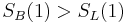 and
and 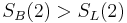 we feel that
  must be greater than
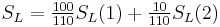
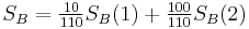
  . However if different weights are used to form the overall score for each person then this feeling may be disappointed. Here the first test is weighted
  for Lisa and
  for Bart while the weights are reversed on the second test.
By more extreme reweighting Lisa's overall score can be pushed up towards 60% and Bart's down towards 30%.
Lisa is a better editor on average, as her overall success rate is higher. But it is possible to have told the story in a way which would make it appear obvious that Bart is more diligent.
Simpson's paradox shows us an extreme example of the importance of including data about possible confounding variables when attempting to calculate causal relations. Precise criteria for selecting a set of "confounding variables," (i.e., variables that yield correct causal relationships if included in the analysis), is given in Pearl[2] using causal graphs.
While Simpson's paradox often refers to the analysis of count tables, as shown in this example, it also occurs with continuous data:[18] for example, if one fits separated regression lines through two sets of data, the two regression lines may show a positive trend, while a regression line fitted through all data together will show a negative trend, as shown on the picture above.
Vector interpretation
Simpson's paradox can also be illustrated using the 2-dimensional vector space.[19] A success rate of  can be represented by a vector
  , with a slope of . If two rates
  and
and  are combined, as in the examples given above, the result can be represented by the sum of the vectors
  and
and  , which according to the parallelogram rule is the vector
  , with slope
  .
.
Simpson's paradox says that even if a vector  (in blue in the figure) has a smaller slope than another vector
  (in red), and
  has a smaller slope than
  , the sum of the two vectors
  (indicated by "+" in the figure) can still have a larger slope than the sum of the two vectors
  , as shown in the example.
Implications to decision making
The practical significance of Simpson's paradox surfaces in decision making situations where it poses the following dilemma: Which data should we consult in choosing an action, the aggregated or the partitioned? In the Kidney Stone example above, it is clear that if one is diagnosed with "Small Stones" or "Large Stones" the data for the respective subpopulation should be consulted and Treatment A would be preferred to Treatment B. But what if a patient is not diagnosed, and the size of the stone is not known; would it be appropriate to consult the aggregated data and administer Treatment B? This would stand contrary to common sense; a treatment that is preferred both under one condition and under its negation should also be preferred when the condition is unknown.
On the other hand, if the partitioned data is to be preferred a priori, what prevents one from partitioning the data into arbitrary sub-categories (say based on eye color or post-treatment pain) artificially constructed to yield wrong choices of treatments? Pearl[2] shows that, indeed, in many cases it is the aggregated, not the partitioned data that gives the correct choice of action. Worse yet, given the same table, one should sometimes follow the partitioned and sometimes the aggregated data, depending on the story behind the data; with each story dictating its own choice. Pearl[2] considers this to be the real paradox behind Simpson's reversal.
As to why and how a story, not data, should dictate choices, the answer is that it is the story which encodes the causal relationships among the variables. Once we extract these relationships and represent them in a graph called a causal Bayesian network we can test algorithmically whether a given partition, representing confounding variables, gives the correct answer. The test, called "back-door," requires that we check whether the nodes corresponding to the confounding variables intercept certain paths in the graph. This reduces Simpson's Paradox to an exercise in graph theory.
How likely is Simpson’s paradox?
If a 2 × 2 × 2 table, such as in the kidney stone example, is selected at random, the probability is approximately 1/60 that Simpson's paradox will occur purely by chance.[20]
References
- Notes
- References
- ^ Clifford H. Wagner (February 1982). "Simpson's Paradox in Real Life". The American Statistician 36 (1): 46–48. doi:10.2307/2684093. JSTOR 2684093.
- ^ a b c d e f Judea Pearl. Causality: Models, Reasoning, and Inference, Cambridge University Press (2000, 2nd edition 2009). ISBN 0-521-77362-8.
- ^ a b David Freedman, Robert Pisani and Roger Purves. Statistics (4th edition). W.W. Norton, 2007, p. 19. ISBN 13-978-0-393-92972-0.
- ^ David S. Moore and D.S. George P. McCabe (February 2005). "Introduction to the Practice of Statistics" (5th edition). W.H. Freeman & Company. ISBN 0-7167-6282-X.
- ^ Robert L. Wardrop (February 1995). "Simpson's Paradox and the Hot Hand in Basketball". The American Statistician, 49 (1): pp. 24–28.
- ^ Alan Agresti (2002). "Categorical Data Analysis" (Second edition). John Wiley and Sons ISBN 0-471-36093-7
- ^ Simpson, Edward H. (1951). "The Interpretation of Interaction in Contingency Tables". Journal of the Royal Statistical Society, Ser. B 13: 238–241.
- ^ Pearson, Karl; Lee, A.; Bramley-Moore, L. (1899). "Genetic (reproductive) selection: Inheritance of fertility in man". Philosophical Translations of the Royal Statistical Society, Ser. A 173: 534–539.
- ^ G. U. Yule (1903). "Notes on the Theory of Association of Attributes in Statistics". Biometrika 2 (2): 121–134. doi:10.1093/biomet/2.2.121.
- ^ Colin R. Blyth (June 1972). "On Simpson's Paradox and the Sure-Thing Principle". Journal of the American Statistical Association 67 (338): 364–366. doi:10.2307/2284382. JSTOR 2284382.
- ^ I. J. Good, Y. Mittal (June 1987). "The Amalgamation and Geometry of Two-by-Two Contingency Tables". The Annals of Statistics 15 (2): 694–711. doi:10.1214/aos/1176350369. ISSN 0090-5364. JSTOR 2241334.
- ^ C. R. Charig, D. R. Webb, S. R. Payne, O. E. Wickham (29 March 1986). "Comparison of treatment of renal calculi by open surgery, percutaneous nephrolithotomy, and extracorporeal shockwave lithotripsy". Br Med J (Clin Res Ed) 292 (6524): 879–882. doi:10.1136/bmj.292.6524.879. PMC 1339981. PMID 3083922. http://www.pubmedcentral.nih.gov/articlerender.fcgi?tool=pmcentrez&artid=1339981.
- ^ Steven A. Julious and Mark A. Mullee (12/03/1994). "Confounding and Simpson's paradox". BMJ 309 (6967): 1480–1481. PMC 2541623. PMID 7804052. http://bmj.bmjjournals.com/cgi/content/full/309/6967/1480.
- ^ a b c P.J. Bickel, E.A. Hammel and J.W. O'Connell (1975). "Sex Bias in Graduate Admissions: Data From Berkeley". Science 187 (4175): 398–404. doi:10.1126/science.187.4175.398. PMID 17835295. http://www.sciencemag.org/cgi/content/abstract/187/4175/398..
- ^ Wilcox Allen (2006). "The Perils of Birth Weight — A Lesson from Directed Acyclic Graphs". American Journal of Epidemiology 164 (11): 1121–1123. doi:10.1093/aje/kwj276. PMID 16931545. http://aje.oxfordjournals.org/cgi/content/abstract/164/11/1121.
- ^ Ken Ross. "A Mathematician at the Ballpark: Odds and Probabilities for Baseball Fans (Paperback)" Pi Press, 2004. ISBN 0-13-147990-3. 12–13
- ^ Statistics available from http://www.baseball-reference.com/ : Data for Derek Jeter, Data for David Justice.
- ^ John Fox (1997). "Applied Regression Analysis, Linear Models, and Related Methods". Sage Publications. ISBN 0-8039-4540-X. 136–137
- ^ Kocik Jerzy (2001). "Proofs without Words: Simpson's Paradox" (PDF). Mathematics Magazine 74 (5): 399. http://www.math.siu.edu/kocik/papers/simpson2.pdf.
- ^ Marios G. Pavlides and Michael D. Perlman (August 2009). "How Likely is Simpson's Paradox?". The American Statistician 63 (3): 226–233. doi:10.1198/tast.2009.09007.
External links
- Stanford Encyclopedia of Philosophy: "Simpson's Paradox" – by Gary Malinas.
- Earliest known uses of some of the words of mathematics: S
- For a brief history of the origins of the paradox see the entries "Simpson's Paradox" and "Spurious Correlation"
- Pearl, Judea, ""The Art and Science of Cause and Effect." A slide show and tutorial lecture.
- Pearl, Judea, "Simpson's Paradox: An Anatomy" (PDF)
- Short articles by Alexander Bogomolny at cut-the-knot:
- The Wall Street Journal column "The Numbers Guy" for December 2, 2009 dealt with recent instances of Simpson's paradox in the news. Notably a Simpson's paradox in the comparison of unemployment rates of the 2009 recession with the 1983 recession. by Cari Tuna (substituting for regular columnist Carl Bialik)